1. 狭义EM
Reference:[统计学习方法 第二版 第九章]
EM算法是一种迭代算法,1977 年由 Dempster 等人总结提出,用于含有隐变量(hidden variable)的概率模型参数的极大似然估计,或极大后验概率估计。EM算法的每次迭代由两步组成:E 步,求期望(expectation);M 步,求极大(maximization)。所以这一算法称为期望极大算法(expectation maximization algorithm),简称 EM 算法。
1.1 EM 算法的引入
概率模型有时既含有观测变量(observable variable),又含有隐变量或潜在变量(latent variable)。如果概率模型的变量都是观测变量,那么给定数据,可以直接用极大似然估计法,或贝叶斯估计法估计模型参数(此时只有固定的参数未知 )。EM 算法就是含有隐变量的概率模型参数的极大似然估计法,或极大后验概率估计法 。
例1(三硬币模型):假设有 3 枚硬币,分别记作 A,B,C。这些硬币正面出现的概率分别是 π \pi π p p p q q q n n n n = 10 n=10 n = 10 1 , 1 , 0 , 1 , 0 , 0 , 1 , 0 , 1 , 1 1,1,0,1,0,0,1,0,1,1 1 , 1 , 0 , 1 , 0 , 0 , 1 , 0 , 1 , 1 P(y\mid \theta)=\sum_z P(y,z\mid\theta)=\sum_zP(z\mid\theta)P(y\mid z,\theta)=\pi p^y(1-p)^{1-y}+(1-\pi)q^y(1-q)^{1-y} \tag{1}
这里随机变量 y y y z z z θ = ( π , p , q ) \theta=(\pi,p,q) θ = ( π , p , q ) P(Y\mid \theta)=\sum_ZP(Z\mid \theta)P(Y\mid Z, \theta)=\prod_{j=1}^n[\pi p^{y_j}(1-p)^{1-y_j}+(1-\pi)q^{y_j}(1-q)^{1-y_j}]\tag{2}
考虑求模型参数 θ = ( π , p , q ) \theta=(\pi, p, q) θ = ( π , p , q ) \hat\theta=\mathrm{arg} \max_\theta \log P(Y\mid \theta)\tag{3}
这个问题没有解析解,因为 log \log log
E 步:计算在模型参数 π ( i ) , p ( i ) , q ( i ) \pi^{(i)},p^{(i)},q^{(i)} π ( i ) , p ( i ) , q ( i ) y j y_j y j \mu_j^{(i+1)}=\frac{\pi^{(i)}(p^{(i)})^{y_j}(1-p^{(i)})^{1-y_j}}{\pi^{(i)}(p^{(i)})^{y_j}(1-p^{(i)})^{1-y_j}+(1-\pi^{(i)})(q^{(i)})^{y_j}(1-q^{(i)})^{1-y_j}}\tag{4}
M 步:计算模型参数的新估计值
π ( i + 1 ) = 1 n ∑ j = 1 n μ j ( i + 1 ) p ( i + 1 ) = ∑ j = 1 n μ j ( i + 1 ) y j ∑ j = 1 n μ j ( i + 1 ) q ( i + 1 ) = ∑ j = 1 n ( 1 − μ j ( i + 1 ) ) y j ∑ j = 1 n ( 1 − μ j ( i + 1 ) ) (5) \begin{aligned}
& \pi^{(i+1)}=\frac{1}{n}\sum_{j=1}^n \mu_j^{(i+1)} \\
& p^{(i+1)} =\frac{\sum_{j=1}^n \mu_j^{(i+1)} y_j}{\sum_{j=1}^n \mu_{j}^{(i+1)}}\\
& q^{(i+1)} = \frac{\sum_{j=1}^n (1-\mu_j^{(i+1)})y_j}{\sum_{j=1}^n (1-\mu_j^{(i+1)})}
\end{aligned}\tag{5} π ( i + 1 ) = n 1 j = 1 ∑ n μ j ( i + 1 ) p ( i + 1 ) = ∑ j = 1 n μ j ( i + 1 ) ∑ j = 1 n μ j ( i + 1 ) y j q ( i + 1 ) = ∑ j = 1 n ( 1 − μ j ( i + 1 ) ) ∑ j = 1 n ( 1 − μ j ( i + 1 ) ) y j ( 5 ) 按照上述迭代步骤直至收敛,若假设模型参数初值为 π ( 0 ) = 0.5 , p ( 0 ) = 0.5 , q ( 0 ) = 0.5 \pi^{(0)}=0.5, p^{(0)}=0.5, q^{(0)}=0.5 π ( 0 ) = 0.5 , p ( 0 ) = 0.5 , q ( 0 ) = 0.5 π ^ = 0.5 , p ^ = 0.6 , q ^ = 0.6 \hat\pi =0.5, \hat p =0.6, \hat q= 0.6 π ^ = 0.5 , p ^ = 0.6 , q ^ = 0.6 π ( 0 ) = 0.4 , p ( 0 ) = 0.6 , q ( 0 ) = 0.6 \pi^{(0)}=0.4, p^{(0)}=0.6, q^{(0)}=0.6 π ( 0 ) = 0.4 , p ( 0 ) = 0.6 , q ( 0 ) = 0.6 π ^ = 0.4064 , p ^ = 0.5368 , q ^ = 0.6432 \hat\pi =0.4064, \hat p =0.5368, \hat q= 0.6432 π ^ = 0.4064 , p ^ = 0.5368 , q ^ = 0.6432
一般地,用 Y Y Y Z Z Z Y Y Y Z Z Z Y Y Y
首先写出所有观测的似然函数
P(Y \mid \theta) = \prod_{j=1}^n P(y_j \mid \theta) = \prod_{j=1}^n [\pi p + (1-\pi) q]^{y_j} [\pi (1-p)+(1-\pi)(1-q)]^{(1-y_j)} \tag{6}
计算 P ( z j = 1 ∣ y j , θ ( i ) ) P(z_j =1 \mid y_j, \theta^{(i)}) P ( z j = 1 ∣ y j , θ ( i ) ) \mu_j^{(i+1)} = P(z_j = 1 \mid y_j, \theta^{(i)}) = \frac{P(y_j \mid z_j =1,\theta^{(i)})P(z_j =1 \mid \theta^{(i)})}{P(y_j \mid \theta^{(i)})}=\begin{cases} \frac{\pi^{(i)} p^{(i)}}{\pi^{(i)} p ^{(i)} + (1-\pi^{(i)})q^{(i)}} &\quad \text{if } y_j=1\\ \frac{\pi^{(i)} (1-p^{(i)})}{\pi^{(i)} (1-p^{(i)})+ (1-\pi^{(i)})(1-q^{(i)})} &\quad \text{if } y_j=0 \end{cases} \tag{7}
计算完全数据的对数似然函数的期望
Q ( θ ∣ θ ( i ) ) = E P ( Z ∣ Y , θ ( i ) ) [ log P ( Y , Z ∣ θ ) ] = E P ( Z ∣ Y , θ ( i ) ) [ ∑ j = 1 n log P ( y j , z j ∣ θ ) ] = ∑ j = 1 n E P ( z j ∣ y j , θ ( i ) ) [ log P ( y j , z j ∣ θ ) ] = ∑ j = 1 n ∑ z j P ( z j ∣ y j , θ ( i ) ) log P ( y j , z j ∣ θ ) = ∑ j = 1 n [ μ j ( i + 1 ) log ( π p y j ( 1 − p ) ( 1 − y j ) ) + ( 1 − μ j ( i + 1 ) ) log ( ( 1 − π ) q y j ( 1 − q ) ( 1 − y j ) ) ] (8) \begin{aligned}
Q(\theta \mid \theta^{(i)}) = &\mathbb{E}_{P(Z \mid Y, \theta^{(i)})}[\log P(Y,Z \mid \theta)] \\
=& \mathbb{E}_{P(Z\mid Y ,\theta^{(i)})} [\sum_{j=1}^n \log P(y_j, z_j \mid \theta)]\\
=& \sum_{j=1}^n \mathbb{E}_{P(z_j \mid y_j , \theta^{(i)})}[\log P(y_j, z_j \mid \theta)]\\
=& \sum_{j=1}^n \sum_{z_j} P(z_j \mid y_j ,\theta^{(i)}) \log P(y_j, z_j \mid \theta)\\
=& \sum_{j=1}^n \left[\mu_j^{(i+1)} \log \left(\pi p^{y_j} (1-p)^{(1-y_j)}\right) + (1-\mu_j^{(i+1)}) \log \left((1-\pi)q^{y_j}(1-q)^{(1-y_j)}\right)\right] \\
\end{aligned}\tag{8} Q ( θ ∣ θ ( i ) ) = = = = = E P ( Z ∣ Y , θ ( i ) ) [ log P ( Y , Z ∣ θ )] E P ( Z ∣ Y , θ ( i ) ) [ j = 1 ∑ n log P ( y j , z j ∣ θ )] j = 1 ∑ n E P ( z j ∣ y j , θ ( i ) ) [ log P ( y j , z j ∣ θ )] j = 1 ∑ n z j ∑ P ( z j ∣ y j , θ ( i ) ) log P ( y j , z j ∣ θ ) j = 1 ∑ n [ μ j ( i + 1 ) log ( π p y j ( 1 − p ) ( 1 − y j ) ) + ( 1 − μ j ( i + 1 ) ) log ( ( 1 − π ) q y j ( 1 − q ) ( 1 − y j ) ) ] ( 8 ) 对各参数求导,并令其满足一阶条件可得公式(5)(可拆解验证其凹性)。
算法1 (EM 算法):
输入:观测变量数据 Y Y Y Z Z Z P ( Y , Z ∣ θ ) P(Y,Z\mid\theta) P ( Y , Z ∣ θ ) P ( Z ∣ Y , θ ) P(Z\mid Y, \theta) P ( Z ∣ Y , θ ) θ \theta θ θ ( 0 ) \theta^{(0)} θ ( 0 ) θ ( i ) \theta^{(i)} θ ( i ) i i i i + 1 i+1 i + 1 Q(\theta, \theta^{(i)})=E_Z[\log P(Y, Z \mid \theta) \mid Y, \theta^{(i)}]=\sum_Z P(Z\mid Y, \theta^{(i)})\log P(Y,Z\mid \theta)\tag{9}
(3)M 步:求使 Q ( θ , θ ( i ) ) Q(\theta,\theta^{(i)}) Q ( θ , θ ( i ) ) θ \theta θ i + 1 i+1 i + 1 θ ( i + 1 ) \theta^{(i+1)} θ ( i + 1 ) \theta^{(i+1)} =\mathrm{arg} \max_{\theta} Q(\theta, \theta^{(i)})\tag{10}
(4)重复第(2)步和第(3)步,直到收敛。
注意:参数的初值可以任意选择,但 EM 算法对初值是敏感的。
定义1:Q Q Q Q Q Q log P ( Y , Z ∣ θ ) \log P(Y,Z \mid \theta) log P ( Y , Z ∣ θ ) Y Y Y θ ( i ) \theta^{(i)} θ ( i ) Z Z Z P ( Z ∣ Y , θ ( i ) ) P(Z\mid Y, \theta^{(i)}) P ( Z ∣ Y , θ ( i ) ) Q Q Q Q(\theta, \theta^{(i)})=E_Z[\log P(Y, Z \mid \theta) \mid Y, \theta^{(i)}]\tag{11}
1.2 EM 算法的导出(其本质都是对似然 log ( Y ∣ θ ) \log{(Y\mid \theta)} log ( Y ∣ θ )
1.2.1 方法一(正向推导,只需要有进步即可)
Reference:[统计学习方法 第二版 179页]
面对一个含有隐变量的概率模型,目标是极大化观测数据(不完全数据) Y Y Y θ \theta θ L(\theta)=\log P(Y\mid \theta) =\log \sum_Z P(Y,Z\mid \theta)=\log \left( \sum_Z P(Y\mid Z,\theta)P(Z\mid \theta) \right)\tag{12}
上式极大化的主要困难在于未观测数据以及对数里的和(或者积分)。
EM 算法是通过迭代逐步近似极大化 L ( θ ) L(\theta) L ( θ ) i i i θ \theta θ θ ( i ) \theta^{(i)} θ ( i ) θ \theta θ L ( θ ) L(\theta) L ( θ ) L ( θ ) > L ( θ ( i ) ) L(\theta)>L(\theta^{(i)}) L ( θ ) > L ( θ ( i ) ) L(\theta) -L(\theta^{(i)})=\log \left(\sum_Z P(Y\mid Z, \theta)P(Z\mid \theta)\right) - \log P(Y\mid \theta^{(i)})\tag{13}
利用 Jensen 不等式得到其下界:
L ( θ ) − L ( θ ( i ) ) = log ( ∑ Z P ( Z ∣ Y , θ ( i ) ) P ( Y ∣ Z , θ ) P ( Z ∣ θ ) P ( Z ∣ Y , θ ( i ) ) ) − log P ( Y ∣ θ ( i ) ) ≥ ∑ Z P ( Z ∣ Y , θ ( i ) ) log P ( Y ∣ Z , θ ) P ( Z ∣ θ ) P ( Z ∣ Y , θ ( i ) ) − log P ( Y ∣ θ ( i ) ) = ∑ Z P ( Z ∣ Y , θ ( i ) ) log P ( Y ∣ Z , θ ) P ( Z ∣ θ ) P ( Z ∣ Y , θ ( i ) ) − ∑ Z P ( Z ∣ Y , θ ( i ) ) log P ( Y ∣ θ ( i ) ) = ∑ Z P ( Z ∣ Y , θ ( i ) ) log P ( Y ∣ Z , θ ) P ( Z ∣ θ ) P ( Z ∣ Y , θ ( i ) ) P ( Y ∣ θ ( i ) ) (14) \begin{aligned}
L(\theta) -L(\theta^{(i)}) = &\log \left(\sum_Z P(Z\mid Y,\theta^{(i)}) \frac{P(Y\mid Z, \theta)P(Z\mid \theta)}{P(Z\mid Y,\theta^{(i)})} \right)-\log P(Y\mid \theta^{(i)}) \\
\geq & \sum_Z P(Z\mid Y, \theta^{(i)}) \log \frac{P(Y\mid Z, \theta)P(Z\mid \theta)}{P(Z\mid Y, \theta^{(i)})} -\log P(Y\mid \theta^{(i)}) \\
=&\sum_Z P(Z\mid Y, \theta^{(i)}) \log \frac{P(Y\mid Z, \theta)P(Z\mid \theta)}{P(Z\mid Y, \theta^{(i)})} - \sum_Z P(Z\mid Y,\theta^{(i)})\log P(Y\mid \theta^{(i)})\\
=& \sum_Z P(Z\mid Y, \theta^{(i)}) \log \frac{P(Y\mid Z,\theta)P(Z\mid \theta)}{P(Z\mid Y, \theta^{(i)})P(Y\mid \theta^{(i)})}\\
\end{aligned}\tag{14} L ( θ ) − L ( θ ( i ) ) = ≥ = = log ( Z ∑ P ( Z ∣ Y , θ ( i ) ) P ( Z ∣ Y , θ ( i ) ) P ( Y ∣ Z , θ ) P ( Z ∣ θ ) ) − log P ( Y ∣ θ ( i ) ) Z ∑ P ( Z ∣ Y , θ ( i ) ) log P ( Z ∣ Y , θ ( i ) ) P ( Y ∣ Z , θ ) P ( Z ∣ θ ) − log P ( Y ∣ θ ( i ) ) Z ∑ P ( Z ∣ Y , θ ( i ) ) log P ( Z ∣ Y , θ ( i ) ) P ( Y ∣ Z , θ ) P ( Z ∣ θ ) − Z ∑ P ( Z ∣ Y , θ ( i ) ) log P ( Y ∣ θ ( i ) ) Z ∑ P ( Z ∣ Y , θ ( i ) ) log P ( Z ∣ Y , θ ( i ) ) P ( Y ∣ θ ( i ) ) P ( Y ∣ Z , θ ) P ( Z ∣ θ ) ( 14 ) 令
B ( θ , θ ( i ) ) = L ( θ ( i ) ) + ∑ Z P ( Z ∣ Y , θ ( i ) ) log P ( Y ∣ Z , θ ) P ( Z ∣ θ ) P ( Z ∣ Y , θ ( i ) ) P ( Y ∣ θ ( i ) ) (15) \begin{aligned}
B(\theta, \theta^{(i)})=&L(\theta^{(i)})+ \sum_Z P(Z\mid Y, \theta^{(i)}) \log \frac{P(Y\mid Z,\theta)P(Z\mid \theta)}{P(Z\mid Y,\theta^{(i)})P(Y\mid \theta^{(i)})}\tag{15}\\
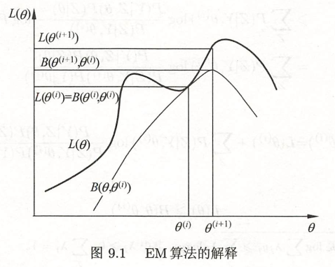
\end{aligned} B ( θ , θ ( i ) ) = L ( θ ( i ) ) + Z ∑ P ( Z ∣ Y , θ ( i ) ) log P ( Z ∣ Y , θ ( i ) ) P ( Y ∣ θ ( i ) ) P ( Y ∣ Z , θ ) P ( Z ∣ θ ) ( 15 ) 则 L ( θ ) ≥ B ( θ , θ ( i ) ) L(\theta) \geq B(\theta, \theta^{(i)}) L ( θ ) ≥ B ( θ , θ ( i ) ) B ( θ , θ ( i ) ) B(\theta, \theta^{(i)}) B ( θ , θ ( i ) ) L ( θ ) L(\theta) L ( θ ) B ( θ ( i ) , θ ( i ) ) = L ( θ ( i ) ) B(\theta^{(i)}, \theta^{(i)}) = L(\theta^{(i)}) B ( θ ( i ) , θ ( i ) ) = L ( θ ( i ) ) B ( θ , θ ( i ) ) B(\theta, \theta^{(i)}) B ( θ , θ ( i ) ) θ ( i ) \theta^{(i)} θ ( i ) θ \theta θ L ( θ ) L(\theta) L ( θ ) L ( θ ( i ) ) = B ( θ ( i ) , θ ( i ) ) ≤ B ( θ ( i + 1 ) , θ ( i ) ) ≤ L ( θ ( i + 1 ) ) L(\theta^{(i)}) = B(\theta^{(i)}, \theta^{(i)})\leq B(\theta^{(i+1)}, \theta^{(i)})\leq L(\theta^{(i+1)}) L ( θ ( i ) ) = B ( θ ( i ) , θ ( i ) ) ≤ B ( θ ( i + 1 ) , θ ( i ) ) ≤ L ( θ ( i + 1 ) )
θ ( i + 1 ) = a r g max θ B ( θ , θ ( i ) ) = a r g max θ ( L ( θ ( i ) ) + ∑ Z P ( Z ∣ Y , θ ( i ) ) log P ( Y ∣ Z , θ ) P ( Z ∣ θ ) P ( Z ∣ Y , θ ( i ) ) P ( Y ∣ θ ( i ) ) ) = a r g max θ ( ∑ Z P ( Z ∣ Y , θ ( i ) ) log P ( Y ∣ Z , θ ) P ( Z ∣ θ ) ) = a r g max θ Q ( θ , θ ( i ) ) (16) \begin{aligned}
\theta^{(i+1)} =& \mathrm{arg} \max_{\theta} B(\theta, \theta^{(i)})\\
=& \mathrm{arg} \max_{\theta} \left(L(\theta^{(i)}) +\sum_Z P(Z\mid Y, \theta^{(i)}) \log \frac{P(Y\mid Z, \theta) P(Z\mid \theta)}{P(Z\mid Y,\theta^{(i)})P(Y\mid \theta^{(i)})} \right)\\
=& \mathrm{arg} \max_{\theta} \left( \sum_Z P(Z\mid Y, \theta^{(i)}) \log P(Y\mid Z, \theta) P(Z\mid \theta)\right)\\
=& \mathrm{arg} \max_{\theta} Q(\theta, \theta^{(i)})\\
\end{aligned}\tag{16} θ ( i + 1 ) = = = = arg θ max B ( θ , θ ( i ) ) arg θ max ( L ( θ ( i ) ) + Z ∑ P ( Z ∣ Y , θ ( i ) ) log P ( Z ∣ Y , θ ( i ) ) P ( Y ∣ θ ( i ) ) P ( Y ∣ Z , θ ) P ( Z ∣ θ ) ) arg θ max ( Z ∑ P ( Z ∣ Y , θ ( i ) ) log P ( Y ∣ Z , θ ) P ( Z ∣ θ ) ) arg θ max Q ( θ , θ ( i ) ) ( 16 ) 下图给出 EM 算法的直观解释:
1.2.2 方法二(通过条件概率公式引入隐变量)
Reference:[变分推断PPT]
对等式两边 log P ( Y ∣ θ ) = log P ( Y , Z ∣ θ ) − log P ( Z ∣ Y , θ ) \log P(Y \mid \theta)=\log P(Y,Z \mid \theta)-\log P(Z \mid Y,\theta) log P ( Y ∣ θ ) = log P ( Y , Z ∣ θ ) − log P ( Z ∣ Y , θ )
左边得到
Left = ∑ Z P ( Z ∣ Y , θ ( i ) ) log P ( Y ∣ θ ) = log P ( Y ∣ θ ) ∑ Z P ( Z ∣ Y , θ ( i ) ) = log P ( Y ∣ θ ) (17) \begin{aligned}
\text{Left} =& \sum_Z P(Z\mid Y,\theta^{(i)})\log P(Y\mid \theta)\\
=& \log P(Y\mid \theta)\sum_Z P(Z\mid Y,\theta^{(i)})\\
=& \log P(Y\mid \theta)\\
\end{aligned}\tag{17} Left = = = Z ∑ P ( Z ∣ Y , θ ( i ) ) log P ( Y ∣ θ ) log P ( Y ∣ θ ) Z ∑ P ( Z ∣ Y , θ ( i ) ) log P ( Y ∣ θ ) ( 17 ) 右边得到
Right = ∑ Z P ( Z ∣ Y , θ ( i ) ) log P ( Y , Z ∣ θ ) − ∑ Z P ( Z ∣ Y , θ ( i ) ) log P ( Z ∣ Y , θ ) = Q ( θ , θ ( i ) ) − H ( θ , θ ( i ) ) (18) \begin{aligned}
\text{Right} =& \sum_Z P(Z\mid Y,\theta^{(i)}) \log P(Y,Z\mid \theta) -\sum_Z P(Z\mid Y,\theta^{(i)}) \log P(Z\mid Y,\theta)\\
=& Q(\theta, \theta^{(i)})- H(\theta, \theta^{(i)})\\
\end{aligned}\tag{18} Right = = Z ∑ P ( Z ∣ Y , θ ( i ) ) log P ( Y , Z ∣ θ ) − Z ∑ P ( Z ∣ Y , θ ( i ) ) log P ( Z ∣ Y , θ ) Q ( θ , θ ( i ) ) − H ( θ , θ ( i ) ) ( 18 ) 此处 Q ( θ , θ ( i ) ) Q(\theta,\theta^{(i)}) Q ( θ , θ ( i ) ) Q ( θ ( i + 1 ) , θ ( i ) ) ≥ Q ( θ ( i ) , θ ( i ) ) Q(\theta^{(i+1)}, \theta^{(i)}) \geq Q(\theta^{(i)}, \theta^{(i)}) Q ( θ ( i + 1 ) , θ ( i ) ) ≥ Q ( θ ( i ) , θ ( i ) )
而对于 H ( θ , θ ( i ) ) H(\theta, \theta^{(i)}) H ( θ , θ ( i ) )
H ( θ ( i + 1 ) , θ ( i ) ) − H ( θ ( i ) , θ ( i ) ) = ∑ Z P ( Z ∣ Y , θ ( i ) ) log P ( Z ∣ Y , θ ( i + 1 ) ) − ∑ Z P ( Z ∣ Y , θ ( i ) ) log P ( Z ∣ Y , θ ( i ) ) = ∑ Z P ( Z ∣ Y , θ ( i ) ) log P ( Z ∣ Y , θ ( i + 1 ) ) P ( Z ∣ Y , θ ( i ) ) ≤ log ∑ Z P ( Z ∣ Y , θ ( i ) ) ⋅ P ( Z ∣ Y , θ ( i + 1 ) ) P ( Z ∣ Y , θ ( i ) ) = 0 (19) \begin{aligned}
&H(\theta^{(i+1)}, \theta^{(i)}) - H(\theta^{(i)}, \theta^{(i)}) \\
=& \sum_Z P(Z\mid Y, \theta^{(i)})\log P(Z\mid Y,\theta^{(i+1)}) - \sum_Z P(Z\mid Y, \theta^{(i)})\log P(Z \mid Y, \theta^{(i)})\\
=& \sum_Z P(Z\mid Y, \theta^{(i)}) \log \frac{P(Z\mid Y, \theta^{(i+1)})}{P(Z\mid Y, \theta^{(i)})}\\
\leq & \log \sum_Z P(Z\mid Y,\theta^{(i)})\cdot \frac{P(Z\mid Y, \theta^{(i+1)})}{P(Z\mid Y, \theta^{(i)})}\\
=& 0\\
\end{aligned}\tag{19} = = ≤ = H ( θ ( i + 1 ) , θ ( i ) ) − H ( θ ( i ) , θ ( i ) ) Z ∑ P ( Z ∣ Y , θ ( i ) ) log P ( Z ∣ Y , θ ( i + 1 ) ) − Z ∑ P ( Z ∣ Y , θ ( i ) ) log P ( Z ∣ Y , θ ( i ) ) Z ∑ P ( Z ∣ Y , θ ( i ) ) log P ( Z ∣ Y , θ ( i ) ) P ( Z ∣ Y , θ ( i + 1 ) ) log Z ∑ P ( Z ∣ Y , θ ( i ) ) ⋅ P ( Z ∣ Y , θ ( i ) ) P ( Z ∣ Y , θ ( i + 1 ) ) 0 ( 19 ) 从而得到
log P ( Y ∣ θ ( i + 1 ) ) − log P ( Y ∣ θ ( i ) ) = [ Q ( θ ( i + 1 ) , θ ( i ) ) − H ( θ ( i + 1 ) , θ ( i ) ) ] − [ Q ( θ ( i ) , θ ( i ) ) − H ( θ ( i ) , θ ( i ) ) ] = [ Q ( θ ( i + 1 ) , θ ( i ) ) − Q ( θ ( i ) , θ ( i ) ) ] − [ H ( θ ( i + 1 ) , θ ( i ) ) − H ( θ ( i ) , θ ( i ) ) ] ≥ 0 (20) \begin{aligned}
& \log P(Y\mid \theta^{(i+1)})-\log P(Y\mid \theta^{(i)}) \\
=& [Q(\theta^{(i+1)}, \theta^{(i)})-H(\theta^{(i+1)}, \theta^{(i)})] - [Q(\theta^{(i)}, \theta^{(i)})-H(\theta^{(i)}, \theta^{(i)})]\\
=& [Q(\theta^{(i+1)}, \theta^{(i)}) - Q(\theta^{(i)}, \theta^{(i)})]-[H(\theta^{(i+1)},\theta^{(i)})-H(\theta^{(i)}, \theta^{(i)})]\\
\geq & 0
\end{aligned}\tag{20} = = ≥ log P ( Y ∣ θ ( i + 1 ) ) − log P ( Y ∣ θ ( i ) ) [ Q ( θ ( i + 1 ) , θ ( i ) ) − H ( θ ( i + 1 ) , θ ( i ) )] − [ Q ( θ ( i ) , θ ( i ) ) − H ( θ ( i ) , θ ( i ) )] [ Q ( θ ( i + 1 ) , θ ( i ) ) − Q ( θ ( i ) , θ ( i ) )] − [ H ( θ ( i + 1 ) , θ ( i ) ) − H ( θ ( i ) , θ ( i ) )] 0 ( 20 ) 1.2.3 方法三(引入隐变量的近似分布,承接变分推断内容)
Reference:[变分推断PPT]
引入隐变量 Z 的某种分布 q ϕ ( Z ) q_{\phi}(Z) q ϕ ( Z )
log P ( Y ∣ θ ) = log P ( Y , Z ∣ θ ) − log P ( Z ∣ Y , θ ) = log P ( Y , Z ∣ θ ) q ( Z ) − log P ( Z ∣ Y , θ ) q ( Z ) (21) \begin{aligned}
\log P(Y \mid \theta) =& \log P(Y,Z\mid \theta) - \log P(Z\mid Y, \theta)\\
=& \log \frac{P(Y,Z \mid \theta)}{q(Z)}-\log \frac{P(Z\mid Y, \theta)}{q(Z)}\\
\end{aligned}\tag{21} log P ( Y ∣ θ ) = = log P ( Y , Z ∣ θ ) − log P ( Z ∣ Y , θ ) log q ( Z ) P ( Y , Z ∣ θ ) − log q ( Z ) P ( Z ∣ Y , θ ) ( 21 ) 对上式两边分别关于分布 q ( Z ) q(Z) q ( Z )
Left = ∑ Z q ( Z ) log P ( Y ∣ θ ) = log P ( Y ∣ θ ) (22) \begin{aligned}
\text{Left} =& \sum_Z q(Z) \log P(Y\mid \theta) \\
=&\log P(Y\mid \theta)\\
\end{aligned}\tag{22} Left = = Z ∑ q ( Z ) log P ( Y ∣ θ ) log P ( Y ∣ θ ) ( 22 ) 右边得到
Right = ∑ Z q ( Z ) log P ( Y , Z ∣ θ ) q ( Z ) − ∑ Z q ( Z ) log P ( Z ∣ Y , θ ) q ( Z ) (23) \begin{aligned}
\text{Right} =& \sum_Z q(Z) \log \frac{P(Y,Z\mid \theta)}{q(Z)} - \sum_Z q(Z) \log \frac{P(Z\mid Y, \theta)}{q(Z)}
\end{aligned}\tag{23} Right = Z ∑ q ( Z ) log q ( Z ) P ( Y , Z ∣ θ ) − Z ∑ q ( Z ) log q ( Z ) P ( Z ∣ Y , θ ) ( 23 ) 联立得到
log P ( Y ∣ θ ) ⏟ evidence = ∑ Z q ( Z ) log P ( Y , Z ∣ θ ) q ( Z ) − ∑ Z q ( Z ) log P ( Z ∣ Y , θ ) q ( Z ) = ∑ Z q ( Z ) log P ( Y , Z ∣ θ ) q ( Z ) ⏟ ELBO + ∑ Z q ( Z ) log q ( Z ) P ( Z ∣ Y , θ ) ⏟ K L ( q ( Z ) ∣ ∣ P ( Z ∣ Y , θ ) ) (24) \begin{aligned}
\underbrace{\log P(Y\mid \theta)}_{\text{evidence}} =& \sum_Z q(Z) \log \frac{P(Y,Z\mid \theta)}{q(Z)} - \sum_Z q(Z) \log \frac{P(Z\mid Y, \theta)}{q(Z)}\\
=& \underbrace{\sum_Z q(Z) \log \frac{P(Y,Z\mid \theta)}{q(Z)}}_{\text{ELBO}} + \underbrace{\sum_Z q(Z) \log \frac{q(Z)}{P(Z\mid Y,\theta)}}_{\mathrm{KL}(q(Z)\mid \mid P\left(Z\mid Y, \theta\right))}\\
\end{aligned}\tag{24} evidence log P ( Y ∣ θ ) = = Z ∑ q ( Z ) log q ( Z ) P ( Y , Z ∣ θ ) − Z ∑ q ( Z ) log q ( Z ) P ( Z ∣ Y , θ ) ELBO Z ∑ q ( Z ) log q ( Z ) P ( Y , Z ∣ θ ) + KL ( q ( Z ) ∣∣ P ( Z ∣ Y , θ ) ) Z ∑ q ( Z ) log P ( Z ∣ Y , θ ) q ( Z ) ( 24 )
log P ( Y ∣ θ ) \log P(Y\mid \theta) log P ( Y ∣ θ ) ∑ Z q ( Z ) log P ( Y , Z ∣ θ ) q ( Z ) \sum_Z q(Z)\log \frac{P(Y,Z\mid \theta)}{q(Z)} ∑ Z q ( Z ) log q ( Z ) P ( Y , Z ∣ θ ) ∑ Z q ( Z ) log q ( Z ) P ( Z ∣ Y , θ ) = K L ( q ( Z ) ∣ ∣ P ( Z ∣ Y , θ ) ) \sum_Z q(Z) \log \frac{q(Z)}{P(Z\mid Y,\theta)} = KL(q(Z)\mid \mid P(Z\mid Y,\theta)) ∑ Z q ( Z ) log P ( Z ∣ Y , θ ) q ( Z ) = K L ( q ( Z ) ∣∣ P ( Z ∣ Y , θ )) q ( Z ) q(Z) q ( Z ) P ( Z ∣ Y , θ ) P(Z\mid Y,\theta) P ( Z ∣ Y , θ )
因为 KL 散度非负,从而得到下式,当且仅当 q ( Z ) = P ( Z ∣ Y , θ ) q(Z) = P(Z\mid Y,\theta) q ( Z ) = P ( Z ∣ Y , θ )
log P ( Y ∣ θ ) ⏟ evidence ≥ ∑ Z q ( Z ) log P ( Y , Z ∣ θ ) q ( Z ) ⏟ ELBO (25) \begin{aligned}
\underbrace{\log P(Y\mid \theta)}_{\text{evidence}} \geq \underbrace{\sum_Z q(Z) \log \frac{P(Y,Z\mid \theta)}{q(Z)}}_{\text{ELBO}}
\end{aligned}\tag{25} evidence log P ( Y ∣ θ ) ≥ ELBO Z ∑ q ( Z ) log q ( Z ) P ( Y , Z ∣ θ ) ( 25 ) E 步:固定参数 θ ( i ) \theta^{(i)} θ ( i ) q ( Z ) = P ( Z ∣ Y , θ ( i ) ) q(Z) =P(Z\mid Y, \theta^{(i)}) q ( Z ) = P ( Z ∣ Y , θ ( i ) ) 不严谨,为何此时取等号,疑为ppt错误 )
log P ( Y ∣ θ ) ⏟ evidence = ∑ Z P ( Z ∣ Y , θ ( i ) ) log P ( Y , Z ∣ θ ) P ( Z ∣ Y , θ ( i ) ) ⏟ ELBO (26) \underbrace{\log P(Y\mid \theta)}_{\text{evidence}} = \underbrace{\sum_Z P(Z\mid Y, \theta^{(i)}) \log \frac{P(Y,Z\mid \theta)}{P(Z\mid Y,\theta^{(i)})}}_{\text{ELBO}}\tag{26} evidence log P ( Y ∣ θ ) = ELBO Z ∑ P ( Z ∣ Y , θ ( i ) ) log P ( Z ∣ Y , θ ( i ) ) P ( Y , Z ∣ θ ) ( 26 ) M 步:ELBO 关于参数 θ \theta θ
θ ( i + 1 ) = a r g max θ ∑ Z P ( Z ∣ Y , θ ( i ) ) log P ( Y , Z ∣ θ ) P ( Z ∣ Y , θ ( i ) ) = a r g max θ ∑ Z P ( Z ∣ Y , θ ( i ) ) log P ( Y , Z ∣ θ ) ⏟ Q ( θ , θ ( i ) ) (27) \begin{aligned}
\theta^{(i+1)} =& \mathrm{arg} \max_{\theta} \sum_Z P(Z\mid Y,\theta^{(i)}) \log \frac{P(Y,Z\mid \theta)}{P(Z\mid Y,\theta^{(i)})} \\
=& \mathrm{arg} \max_{\theta} \underbrace{\sum_Z P(Z\mid Y, \theta^{(i)}) \log P(Y,Z\mid \theta)}_{Q(\theta, \theta^{(i)})}\\
\end{aligned}\tag{27} θ ( i + 1 ) = = arg θ max Z ∑ P ( Z ∣ Y , θ ( i ) ) log P ( Z ∣ Y , θ ( i ) ) P ( Y , Z ∣ θ ) arg θ max Q ( θ , θ ( i ) ) Z ∑ P ( Z ∣ Y , θ ( i ) ) log P ( Y , Z ∣ θ ) ( 27 ) 笔者更正:固定参数 θ ( i ) \theta^{(i)} θ ( i ) q ( Z ) = P ( Z ∣ Y , θ ( i ) ) q(Z) =P(Z\mid Y, \theta^{(i)}) q ( Z ) = P ( Z ∣ Y , θ ( i ) )
log P ( Y ∣ θ ) = ∑ Z P ( Z ∣ Y , θ ( i ) ) log P ( Y , Z ∣ θ ) P ( Z ∣ Y , θ ( i ) ) ⏟ A + ∑ Z P ( Z ∣ Y , θ ( i ) ) log P ( Z ∣ Y , θ ( i ) ) P ( Z ∣ Y , θ ) ⏟ B (28) \log P(Y\mid \theta) = \underbrace{\sum_Z P(Z\mid Y, \theta^{(i)}) \log \frac{P(Y,Z\mid \theta)}{P(Z\mid Y,\theta^{(i)})}}_{A} + \underbrace{\sum_Z P(Z\mid Y,\theta^{(i)}) \log \frac{P(Z\mid Y,\theta^{(i)})}{P(Z\mid Y,\theta)}}_{B}\tag{28} log P ( Y ∣ θ ) = A Z ∑ P ( Z ∣ Y , θ ( i ) ) log P ( Z ∣ Y , θ ( i ) ) P ( Y , Z ∣ θ ) + B Z ∑ P ( Z ∣ Y , θ ( i ) ) log P ( Z ∣ Y , θ ) P ( Z ∣ Y , θ ( i ) ) ( 28 ) 而当θ = θ ( i ) \theta = \theta^{(i)} θ = θ ( i )
log P ( Y ∣ θ ( i ) ) = ∑ Z P ( Z ∣ Y , θ ( i ) ) log P ( Y , Z ∣ θ ( i ) ) P ( Z ∣ Y , θ ( i ) ) ⏟ C + ∑ Z P ( Z ∣ Y , θ ( i ) ) log P ( Z ∣ Y , θ ( i ) ) P ( Z ∣ Y , θ ( i ) ) ⏟ D (29) \log P(Y\mid \theta^{(i)}) = \underbrace{\sum_Z P(Z\mid Y, \theta^{(i)}) \log \frac{P(Y,Z\mid \theta^{(i)})}{P(Z\mid Y,\theta^{(i)})}}_{C} + \underbrace{\sum_Z P(Z\mid Y,\theta^{(i)}) \log \frac{P(Z\mid Y,\theta^{(i)})}{P(Z\mid Y,\theta^{(i)})}}_{D}\tag{29} log P ( Y ∣ θ ( i ) ) = C Z ∑ P ( Z ∣ Y , θ ( i ) ) log P ( Z ∣ Y , θ ( i ) ) P ( Y , Z ∣ θ ( i ) ) + D Z ∑ P ( Z ∣ Y , θ ( i ) ) log P ( Z ∣ Y , θ ( i ) ) P ( Z ∣ Y , θ ( i ) ) ( 29 ) 由KL散度性质可知 B ≥ D = 0 B\geq D=0 B ≥ D = 0
θ ( i + 1 ) = arg max θ ∑ Z P ( Z ∣ Y , θ ( i ) ) log P ( Y , Z ∣ θ ) ⏟ Q ( θ , θ ( i ) ) = arg max θ A ⇒ A ( θ ( i + 1 ) ) ≥ C ⇒ log P ( Y ∣ θ ( i + 1 ) ) ≥ log P ( Y ∣ θ ( i ) ) (30) \begin{aligned}
\theta^{(i+1)} &=\arg \max_{\theta} \underbrace{\sum_Z P(Z\mid Y,\theta^{(i)}) \log P(Y,Z\mid \theta) }_{Q(\theta,\theta^{(i)})} \\
&=\arg \max_{\theta} A \\
\Rightarrow \quad \quad & A(\theta^{(i+1)}) \geq C \\
\Rightarrow \quad \quad & \log P(Y\mid \theta^{(i+1)}) \geq \log P(Y\mid \theta^{(i)})
\end{aligned}\tag{30} θ ( i + 1 ) ⇒ ⇒ = arg θ max Q ( θ , θ ( i ) ) Z ∑ P ( Z ∣ Y , θ ( i ) ) log P ( Y , Z ∣ θ ) = arg θ max A A ( θ ( i + 1 ) ) ≥ C log P ( Y ∣ θ ( i + 1 ) ) ≥ log P ( Y ∣ θ ( i ) ) ( 30 ) 1.3 EM 算法的收敛性
定理1:设 L ( θ ) = log P ( Y ∣ θ ) L(\theta)=\log P(Y \mid \theta) L ( θ ) = log P ( Y ∣ θ ) θ ( i ) ( i = 1 , 2 , ⋯ ) \theta^{(i)}(i=1,2, \cdots) θ ( i ) ( i = 1 , 2 , ⋯ ) L ( θ ( i ) ) ( i = 1 , 2 , ⋯ ) L\left(\theta^{(i)}\right)(i=1,2, \cdots) L ( θ ( i ) ) ( i = 1 , 2 , ⋯ ) P ( Y ∣ θ ) P(Y \mid \theta) P ( Y ∣ θ ) L ( θ ( i ) ) = log P ( Y ∣ θ ( i ) ) L\left(\theta^{(i)}\right)=\log P\left(Y \mid \theta^{(i)}\right) L ( θ ( i ) ) = log P ( Y ∣ θ ( i ) ) L ∗ L^* L ∗ 在函数 Q ( θ , θ ′ ) \color{red}{Q\left(\theta, \theta^{\prime}\right)} Q ( θ , θ ′ ) L ( θ ) \color{red}{L(\theta)} L ( θ ) ,由 EM 算法得到的参数估计序列 θ ( i ) \theta^{(i)} θ ( i ) θ ∗ \theta^* θ ∗ L ( θ ) L(\theta) L ( θ )
证明:
(1) 由 L ( θ ( i ) ) = log P ( Y ∣ θ ( i ) ) L(\theta^{(i)})=\log P\left(Y \mid \theta^{(i)}\right) L ( θ ( i ) ) = log P ( Y ∣ θ ( i ) ) P ( Y ∣ θ ) P(Y \mid \theta) P ( Y ∣ θ )
1.4 EM 算法在高斯混合模型学习中的应用
定义2:高斯混合模型
高斯混合模型是指具有如下形式的概率分布模型:
P(y\mid \theta) =\sum_{k=1}^K \alpha_k \cdot \phi(y\mid \theta_k)\tag{31}
其中,α k \alpha_k α k α k ≥ 0 \alpha_k \geq 0 α k ≥ 0 ∑ k = 1 K α k = 1 \sum_{k=1}^K \alpha_k = 1 ∑ k = 1 K α k = 1 ϕ ( y ∣ θ k ) \phi(y \mid \theta_k) ϕ ( y ∣ θ k ) θ k = ( μ k , σ k 2 ) \theta_k = (\mu_k,\sigma_k^2) θ k = ( μ k , σ k 2 ) \phi(y\mid \theta_k) = \frac{1}{\sqrt{2 \pi} \sigma_k} \exp{\left(-\frac{(y-\mu_k)^2}{2\sigma_k^2}\right)}\tag{32}
称为第 k k k
1.4.1 高斯混合模型参数估计的 EM 算法
假设观测数据 y 1 , y 2 , … , y N y_1,y_2,\dots,y_N y 1 , y 2 , … , y N P(y\mid \theta) = \sum_{k=1}^K \alpha_k \cdot \phi(y\mid \theta_k) \tag{33}
其中,θ = ( α 1 , α 2 , … , α K ; θ 1 , θ 2 , … , θ K ) \theta = (\alpha_1,\alpha_2,\dots,\alpha_K;\theta_1,\theta_2,\dots,\theta_K) θ = ( α 1 , α 2 , … , α K ; θ 1 , θ 2 , … , θ K )
观测数据的产生过程:首先依概率 ( α 1 , … , α K ) (\alpha_1,\dots,\alpha_K) ( α 1 , … , α K ) k k k k k k ϕ ( y ∣ θ k ) \phi(y\mid \theta_k) ϕ ( y ∣ θ k ) y j y_j y j y j y_j y j j = 1 , 2 , … , N j=1,2,\dots,N j = 1 , 2 , … , N y j y_j y j k k k k = 1 , 2 , … , K k=1,2,\dots,K k = 1 , 2 , … , K γ j k \gamma_{jk} γ j k \gamma_{jk}=\begin{cases} 1, &\quad \text{第 } j \text{ 个观测来自第 } k \text{ 个分模型} \\ 0, &\quad \text{否则} \end{cases}\tag{34}
有了观测数据 y j y_j y j γ j k \gamma_{jk} γ j k (y_j,\gamma_{j1},\gamma_{j2},\dots,\gamma_{jK}), \quad j=1,2,\dots,N \tag{35}
于是可以写出完全数据的似然函数
P ( y , γ ∣ θ ) = ∏ j = 1 N P ( y j , γ j 1 , γ j 2 , … , γ j K ∣ θ ) = ∏ k = 1 K ∏ j = 1 N [ α k ⋅ ϕ ( y j ∣ θ k ) ] γ j k = ∏ k = 1 K α k n k ∏ j = 1 N [ ϕ ( y j ∣ θ k ) ] γ j k = ∏ k = 1 K α k n k ∏ j = 1 N [ 1 2 π σ k exp ( − ( y j − μ k ) 2 2 σ k 2 ) ] γ j k (36) \begin{aligned}
P(y,\gamma\mid \theta)&=\prod_{j=1}^N P(y_j,\gamma_{j1},\gamma_{j2},\dots,\gamma_{jK} \mid \theta)\\
&=\prod_{k=1}^K \prod_{j=1}^N[\alpha_k \cdot \phi(y_j \mid \theta_k)]^{\gamma_{jk}}\\
&=\prod_{k=1}^K \alpha_k^{n_k} \prod_{j=1}^N [\phi(y_j\mid \theta_k)]^{\gamma_{jk}}\\
&=\prod_{k=1}^K \alpha_k^{n_k} \prod_{j=1}^N \left[\frac{1}{\sqrt{2\pi}\sigma_k}\exp{\left(-\frac{(y_j-\mu_k)^2}{2\sigma_k^2}\right)} \right]^{\gamma_{jk}}
\end{aligned}\tag{36} P ( y , γ ∣ θ ) = j = 1 ∏ N P ( y j , γ j 1 , γ j 2 , … , γ j K ∣ θ ) = k = 1 ∏ K j = 1 ∏ N [ α k ⋅ ϕ ( y j ∣ θ k ) ] γ j k = k = 1 ∏ K α k n k j = 1 ∏ N [ ϕ ( y j ∣ θ k ) ] γ j k = k = 1 ∏ K α k n k j = 1 ∏ N [ 2 π σ k 1 exp ( − 2 σ k 2 ( y j − μ k ) 2 ) ] γ j k ( 36 ) 式中,n k = ∑ j = 1 N γ j k n_k=\sum_{j=1}^N \gamma_{jk} n k = ∑ j = 1 N γ j k ∑ k = 1 K n k = N \sum_{k=1}^K n_k =N ∑ k = 1 K n k = N
那么,完全数据的对数似然函数为
\log P(y, \gamma \mid \theta)=\sum_{k=1}^K\left\{n_k \log \alpha_k+\sum_{j=1}^N \gamma_{j k}\left[\log \left(\frac{1}{\sqrt{2 \pi}}\right)-\log \sigma_k-\frac{1}{2 \sigma_k^2}\left(y_j-\mu_k\right)^2\right]\right\}\tag{37}
进一步计算 Q 函数
Q ( θ , θ ( i ) ) = E γ [ log P ( y , γ ∣ θ ) ∣ y , θ ( i ) ] = E γ { ∑ k = 1 K { n k log α k + ∑ j = 1 N γ j k [ log ( 1 2 π ) − log σ k − 1 2 σ k 2 ( y j − μ k ) 2 ] } } = ∑ k = 1 K { ∑ j = 1 N ( E [ γ j k ] ) log α k + ∑ j = 1 N ( E [ γ j k ] ) [ log ( 1 2 π ) − log σ k − 1 2 σ k 2 ( y j − μ k ) 2 ] } (38) \begin{aligned}
Q(\theta, \theta^{(i)}) & =E_{\gamma}\left[\log P(y, \gamma \mid \theta) \mid y, \theta^{(i)}\right] \\
& =E_{\gamma}\left\{\sum_{k=1}^K\left\{n_k \log \alpha_k+\sum_{j=1}^N \gamma_{j k}\left[\log \left(\frac{1}{\sqrt{2 \pi}}\right)-\log \sigma_k-\frac{1}{2 \sigma_k^2}\left(y_j-\mu_k\right)^2\right]\right\}\right\} \\
& =\sum_{k=1}^K\left\{\sum_{j=1}^N\left(E [\gamma_{j k}]\right) \log \alpha_k+\sum_{j=1}^N\left(E [\gamma_{jk}]\right)\left[\log \left(\frac{1}{\sqrt{2 \pi}}\right)-\log \sigma_k-\frac{1}{2 \sigma_k^2}\left(y_j-\mu_k\right)^2\right]\right\}
\end{aligned}\tag{38} Q ( θ , θ ( i ) ) = E γ [ log P ( y , γ ∣ θ ) ∣ y , θ ( i ) ] = E γ { k = 1 ∑ K { n k log α k + j = 1 ∑ N γ j k [ log ( 2 π 1 ) − log σ k − 2 σ k 2 1 ( y j − μ k ) 2 ] } } = k = 1 ∑ K { j = 1 ∑ N ( E [ γ j k ] ) log α k + j = 1 ∑ N ( E [ γ j k ] ) [ log ( 2 π 1 ) − log σ k − 2 σ k 2 1 ( y j − μ k ) 2 ] } ( 38 ) 这里需要计算 E ( γ j k ∣ y , θ ) E(\gamma_{jk} \mid y, \theta) E ( γ j k ∣ y , θ ) γ ^ j k \hat{\gamma}_{jk} γ ^ j k
γ ^ j k = E ( γ j k ∣ y , θ ) = P ( γ j k = 1 ∣ y , θ ) = P ( γ j k = 1 , y j ∣ θ ) ∑ k = 1 K P ( γ j k = 1 , y j ∣ θ ) = P ( y j ∣ γ j k = 1 , θ ) P ( γ j k = 1 ∣ θ ) ∑ k = 1 K P ( y j ∣ γ j k = 1 , θ ) P ( γ j k = 1 ∣ θ ) = α k ϕ ( y j ∣ θ k ) ∑ k = 1 K α k ϕ ( y j ∣ θ k ) , j = 1 , 2 , ⋯ , N ; k = 1 , 2 , ⋯ , K (39) \begin{aligned}
\hat{\gamma}_{j k} & =E\left(\gamma_{j k} \mid y, \theta\right)=P\left(\gamma_{j k}=1 \mid y, \theta\right) \\
& =\frac{P\left(\gamma_{j k}=1, y_j \mid \theta\right)}{\sum_{k=1}^K P\left(\gamma_{j k}=1, y_j \mid \theta\right)}\\
& =\frac{P\left(y_j \mid \gamma_{j k}=1, \theta\right) P\left(\gamma_{j k}=1 \mid \theta\right)}{\sum_{k=1}^K P\left(y_j \mid \gamma_{j k}=1, \theta\right) P\left(\gamma_{j k}=1 \mid \theta\right)} \\
& =\frac{\alpha_k \phi\left(y_j \mid \theta_k\right)}{\sum_{k=1}^K \alpha_k \phi\left(y_j \mid \theta_k\right)}, \quad j=1,2, \cdots, N ; \quad k=1,2, \cdots, K
\end{aligned}\tag{39} γ ^ j k = E ( γ j k ∣ y , θ ) = P ( γ j k = 1 ∣ y , θ ) = ∑ k = 1 K P ( γ j k = 1 , y j ∣ θ ) P ( γ j k = 1 , y j ∣ θ ) = ∑ k = 1 K P ( y j ∣ γ j k = 1 , θ ) P ( γ j k = 1 ∣ θ ) P ( y j ∣ γ j k = 1 , θ ) P ( γ j k = 1 ∣ θ ) = ∑ k = 1 K α k ϕ ( y j ∣ θ k ) α k ϕ ( y j ∣ θ k ) , j = 1 , 2 , ⋯ , N ; k = 1 , 2 , ⋯ , K ( 39 ) γ ^ j k \hat{\gamma}_{jk} γ ^ j k j j j k k k k k k y j y_j y j γ ^ j k = E [ γ j k ] \hat{\gamma}_{jk}=E[{\gamma_{jk}}] γ ^ j k = E [ γ j k ] n ^ k = ∑ j = 1 N E [ γ j k ] \hat{n}_k = \sum_{j=1}^N E[\gamma_{jk}] n ^ k = ∑ j = 1 N E [ γ j k ] Q\left(\theta, \theta^{(i)}\right)=\sum_{k=1}^K\left\{\hat{n}_k \log \alpha_k+\sum_{j=1}^N \hat{\gamma}_{j k}\left[\log \left(\frac{1}{\sqrt{2 \pi}}\right)-\log \sigma_k-\frac{1}{2 \sigma_k^2}\left(y_j-\mu_k\right)^2\right]\right\}\tag{40}
迭代的 M 步是求函数 Q ( θ , θ ( i ) ) Q(\theta, \theta^{(i)}) Q ( θ , θ ( i ) ) θ \theta θ \theta^{(i+1)} = \arg \max_{\theta} Q(\theta, \theta^{(i)})\tag{41}
用 μ ^ k \hat{\mu}_k μ ^ k σ ^ k 2 \hat{\sigma}_{k}^2 σ ^ k 2 α ^ k \hat{\alpha}_k α ^ k k = 1 , 2 , … , K k=1,2,\dots, K k = 1 , 2 , … , K θ ( i + 1 ) \theta^{(i+1)} θ ( i + 1 ) μ ^ k \hat{\mu}_k μ ^ k σ ^ k 2 \hat{\sigma}_{k}^2 σ ^ k 2 μ ^ k \hat{\mu}_k μ ^ k σ ^ k 2 \hat{\sigma}_{k}^2 σ ^ k 2 α ^ k \hat{\alpha}_k α ^ k ∑ k = 1 K α k = 1 \sum_{k=1}^K \alpha_k=1 ∑ k = 1 K α k = 1 \hat{\mu}_k = \frac{\sum_{j=1}^N \hat{\gamma}_{jk} \cdot y_j}{\sum_{j=1}^N \hat{\gamma}_{jk}}, \quad k=1,2,\dots,K \tag{42}
\hat{\sigma}_{k}^2 =\frac{\sum_{j=1}^N \hat{\gamma}_{jk} (y_j-\mu_k)^2}{\sum_{j=1}^N \hat{\gamma}_{jk}}, \quad k=1,2,\dots,K \tag{43}
\hat{\alpha}_k = \frac{\hat{n}_k}{N} =\frac{\sum_{j=1}^N \hat{\gamma}_{jk}}{N}, \quad k=1,2,\dots, K \tag{44}
重复以上计算,直到对数似然函数值不再有明显的变化为止。
1.5 EM 算法的推广(可参考变分推断PPT更简单易理解)
1.5.1 F 函数的极大-极大算法
定义3:F 函数
假设隐变量数据 Z Z Z P ~ ( Z ) \tilde{P}(Z) P ~ ( Z ) P ~ \tilde{P} P ~ θ \theta θ F ( P ~ , θ ) F(\tilde{P},\theta) F ( P ~ , θ ) F(\tilde{P},\theta)=E_{\tilde{P}}[\log P(Y,Z\mid \theta)]+H(\tilde{P}) \tag{45}
称为 F F F H ( P ~ ) = − E P ~ log P ~ ( Z ) H(\tilde{P})=-E_{\tilde{P}}\log \tilde{P}(Z) H ( P ~ ) = − E P ~ log P ~ ( Z ) P ~ ( Z ) \tilde{P}(Z) P ~ ( Z )
在定义3中,通常假设 P ( Y , Z ∣ θ ) P(Y,Z\mid \theta) P ( Y , Z ∣ θ ) θ \theta θ F ( P ~ , θ ) F(\tilde{P},\theta) F ( P ~ , θ ) P ~ \tilde{P} P ~ θ \theta θ F ( P ~ , θ ) F(\tilde{P}, \theta) F ( P ~ , θ ) θ \theta θ P ~ θ \tilde{P}_{\theta} P ~ θ F ( P ~ , θ ) F(\tilde{P},\theta) F ( P ~ , θ ) P ~ θ \tilde{P}_{\theta} P ~ θ \tilde{P}_{\theta}(Z)=P(Z\mid Y,\theta) \tag{46}
并且 P ~ θ \tilde{P}_{\theta} P ~ θ θ \theta θ
证明:
对于固定的 θ \theta θ F ( P ~ , θ ) F(\tilde{P},\theta) F ( P ~ , θ ) P ~ θ ( Z ) \tilde{P}_{\theta}(Z) P ~ θ ( Z ) λ \lambda λ L=E_{\tilde{P}}\log P(Y,Z\mid \theta)-E_{\tilde{P}}\log \tilde{P}(Z) + \lambda \left(1- \sum_Z \tilde{P}(Z)\right)\tag{47}
将其对 P ~ \tilde{P} P ~ Z Z Z \frac{\partial L}{\partial \tilde{P}(Z)}=\log P(Y,Z\mid \theta)-\log \tilde{P}(Z) -1-\lambda \tag{48}
令偏导数等于 0,得出
\lambda=\log P(Y,Z\mid \theta)-\log \tilde{P}_{\theta}(Z)-1 \tag{49}
由此推出 P ~ θ ( Z ) \tilde{P}_{\theta}(Z) P ~ θ ( Z ) P ( Y , Z ∣ θ ) P(Y,Z\mid \theta) P ( Y , Z ∣ θ ) \frac{P(Y,Z\mid \theta)}{\tilde{P}_{\theta}(Z)}=\exp{(1+\lambda)} \tag{50}
再从约束条件 ∑ Z P ~ θ ( Z ) = 1 \sum_Z \tilde{P}_{\theta}(Z)=1 ∑ Z P ~ θ ( Z ) = 1 P ( Y , Z ∣ θ ) P(Y,Z\mid\theta) P ( Y , Z ∣ θ ) θ \theta θ P ~ θ \tilde{P}_{\theta} P ~ θ θ \theta θ
引理2:
若 P ~ θ ( Z ) = P ( Z ∣ Y , θ ) \tilde{P}_{\theta}(Z)=P(Z\mid Y,\theta) P ~ θ ( Z ) = P ( Z ∣ Y , θ ) F(\tilde{P},\theta)=\log P(Y\mid \theta) \tag{51}
证明:
F ( P ~ , θ ) = E P ~ [ log P ( Y , Z ∣ θ ) ] + H ( P ~ ) = E P ~ [ log P ( Y , Z ∣ θ ) P ( Z ∣ Y , θ ) ] = ∑ Z P ( Z ∣ Y , θ ) ⋅ log P ( Y , Z ∣ θ ) P ( Z ∣ Y , θ ) = ∑ Z P ( Z ∣ Y , θ ) ⋅ log P ( Y ∣ θ ) = log P ( Y ∣ θ ) (52) \begin{aligned}
F(\tilde{P},\theta)=&E_{\tilde{P}}[\log P(Y,Z\mid \theta)]+H(\tilde{P})\\
=&E_{\tilde{P}}[\log \frac{P(Y,Z\mid\theta)}{P(Z\mid Y,\theta)}]\\
=&\sum_Z P(Z\mid Y,\theta)\cdot \log \frac{P(Y,Z\mid\theta)}{P(Z\mid Y,\theta)} \\
=&\sum_Z P(Z\mid Y,\theta) \cdot \log P(Y\mid \theta) \\
=&\log P(Y\mid \theta)
\end{aligned}\tag{52} F ( P ~ , θ ) = = = = = E P ~ [ log P ( Y , Z ∣ θ )] + H ( P ~ ) E P ~ [ log P ( Z ∣ Y , θ ) P ( Y , Z ∣ θ ) ] Z ∑ P ( Z ∣ Y , θ ) ⋅ log P ( Z ∣ Y , θ ) P ( Y , Z ∣ θ ) Z ∑ P ( Z ∣ Y , θ ) ⋅ log P ( Y ∣ θ ) log P ( Y ∣ θ ) ( 52 ) 由以上引理,可以得到关于 EM 算法用 F F F L ( θ ) = log P ( Y ∣ θ ) L(\theta)=\log P(Y\mid \theta) L ( θ ) = log P ( Y ∣ θ ) θ ( i ) , i = 1 , 2 , … \theta^{(i)}, i=1,2,\dots θ ( i ) , i = 1 , 2 , … F ( P ~ , θ ) F(\tilde{P},\theta) F ( P ~ , θ ) F ( P ~ , θ ) F(\tilde{P},\theta) F ( P ~ , θ ) P ~ ∗ \tilde{P}^* P ~ ∗ θ ∗ \theta^* θ ∗ L ( θ ) L(\theta) L ( θ ) θ ∗ \theta^* θ ∗ F ( P ~ , θ ) F(\tilde{P},\theta) F ( P ~ , θ ) P ~ ∗ \tilde{P}^* P ~ ∗ θ ∗ \theta^* θ ∗ L ( θ ) L(\theta) L ( θ ) θ ∗ \theta^* θ ∗ L ( θ ) = log P ( Y ∣ θ ) = F ( P ~ θ , θ ) L(\theta)=\log P(Y\mid \theta)=F(\tilde{P}_{\theta},\theta) L ( θ ) = log P ( Y ∣ θ ) = F ( P ~ θ , θ ) 对任意 θ \color{red}{\theta} θ 。特别地,对于使 F ( P ~ , θ ) F(\tilde{P},\theta) F ( P ~ , θ ) θ ∗ \theta^* θ ∗ L(\theta^*)=F(\tilde{P}_{\theta^*}, \theta^*)=F(\tilde{P}^*, \theta^*)\tag{53}
为了证明 θ ∗ \theta^* θ ∗ L ( θ ) L(\theta) L ( θ ) θ ∗ \theta^* θ ∗ θ ∗ ∗ \theta^{**} θ ∗∗ L ( θ ∗ ∗ ) > L ( θ ∗ ) L(\theta^{**})>L(\theta^*) L ( θ ∗∗ ) > L ( θ ∗ ) θ ∗ ∗ \theta^{**} θ ∗∗ F ( P ~ ∗ ∗ , θ ∗ ∗ ) > F ( P ~ ∗ , θ ∗ ) F(\tilde{P}^{**},\theta^{**})>F(\tilde{P}^*,\theta^*) F ( P ~ ∗∗ , θ ∗∗ ) > F ( P ~ ∗ , θ ∗ ) P ~ ∗ ∗ = P ~ θ ∗ ∗ \tilde{P}^{**}=\tilde{P}_{\theta^{**}} P ~ ∗∗ = P ~ θ ∗∗ P ~ θ \tilde{P}_{\theta} P ~ θ θ \theta θ P ~ ∗ ∗ \tilde{P}^{**} P ~ ∗∗ P ~ ∗ \tilde{P}^* P ~ ∗ P ~ ∗ \tilde{P}^* P ~ ∗ θ ∗ \theta^* θ ∗ F ( P ~ , θ ) F(\tilde{P},\theta) F ( P ~ , θ )
定理3:
EM 算法的一次迭代可由 F F F θ ( i ) \theta^{(i)} θ ( i ) i i i θ \theta θ P ~ ( i ) \tilde{P}^{(i)} P ~ ( i ) i i i P ~ \tilde{P} P ~ i + 1 i+1 i + 1 θ ( i ) \theta^{(i)} θ ( i ) P ~ ( i + 1 ) \tilde{P}^{(i+1)} P ~ ( i + 1 ) F ( P ~ , θ ( i ) ) F\left(\tilde{P}, \theta^{(i)}\right) F ( P ~ , θ ( i ) ) P ~ ( i + 1 ) \tilde{P}^{(i+1)} P ~ ( i + 1 ) θ ( i + 1 ) \theta^{(i+1)} θ ( i + 1 ) F ( P ~ ( i + 1 ) , θ ) F\left(\tilde{P}^{(i+1)}, \theta\right) F ( P ~ ( i + 1 ) , θ ) θ ( i ) \theta^{(i)} θ ( i )
P ~ ( i + 1 ) ( Z ) = P ~ θ ( i ) ( Z ) = P ( Z ∣ Y , θ ( i ) ) (54) \tilde{P}^{(i+1)}(Z)=\tilde{P}_{\theta^{(i)}}(Z)=P(Z \mid Y, \theta^{(i)}) \tag{54} P ~ ( i + 1 ) ( Z ) = P ~ θ ( i ) ( Z ) = P ( Z ∣ Y , θ ( i ) ) ( 54 ) 使 F ( P ~ , θ ( i ) ) F(\tilde{P}, \theta^{(i)}) F ( P ~ , θ ( i ) )
F ( P ~ ( i + 1 ) , θ ) = E P ~ ( i + 1 ) [ log P ( Y , Z ∣ θ ) ] + H ( P ~ ( i + 1 ) ) = ∑ Z log P ( Y , Z ∣ θ ) P ( Z ∣ Y , θ ( i ) ) + H ( P ~ ( i + 1 ) ) (55) \begin{aligned}
F(\tilde{P}^{(i+1)}, \theta) & =E_{\tilde{P}^{(i+1)}}[\log P(Y, Z \mid \theta)]+H(\tilde{P}^{(i+1)}) \\
& =\sum_Z \log P(Y, Z \mid \theta) P(Z \mid Y, \theta^{(i)})+H(\tilde{P}^{(i+1)})
\end{aligned}\tag{55} F ( P ~ ( i + 1 ) , θ ) = E P ~ ( i + 1 ) [ log P ( Y , Z ∣ θ )] + H ( P ~ ( i + 1 ) ) = Z ∑ log P ( Y , Z ∣ θ ) P ( Z ∣ Y , θ ( i ) ) + H ( P ~ ( i + 1 ) ) ( 55 ) 由 Q ( θ , θ ( i ) ) Q\left(\theta, \theta^{(i)}\right) Q ( θ , θ ( i ) )
F ( P ~ ( i + 1 ) , θ ) = Q ( θ , θ ( i ) ) + H ( P ~ ( i + 1 ) ) (56) F\left(\tilde{P}^{(i+1)}, \theta\right)=Q\left(\theta, \theta^{(i)}\right)+H\left(\tilde{P}^{(i+1)}\right)\tag{56} F ( P ~ ( i + 1 ) , θ ) = Q ( θ , θ ( i ) ) + H ( P ~ ( i + 1 ) ) ( 56 ) (2) 固定 P ~ ( i + 1 ) \tilde{P}^{(i+1)} P ~ ( i + 1 ) θ ( i + 1 ) \theta^{(i+1)} θ ( i + 1 ) F ( P ~ ( i + 1 ) , θ ) F\left(\tilde{P}^{(i+1)}, \theta\right) F ( P ~ ( i + 1 ) , θ )
θ ( i + 1 ) = arg max θ F ( P ~ ( i + 1 ) , θ ) = arg max θ Q ( θ , θ ( i ) ) (57) \theta^{(i+1)}=\arg \max _\theta F\left(\tilde{P}^{(i+1)}, \theta\right)=\arg \max _\theta Q\left(\theta, \theta^{(i)}\right)\tag{57} θ ( i + 1 ) = arg θ max F ( P ~ ( i + 1 ) , θ ) = arg θ max Q ( θ , θ ( i ) ) ( 57 ) 通过以上两步完成了 EM 算法的一次迭代。由此可知,由 EM算法与 F F F θ ( i ) , i = 1 , 2 , ⋯ \theta^{(i)}, i=1,2, \cdots θ ( i ) , i = 1 , 2 , ⋯
1.5.2 GEM 算法
算法2:
输入:观测数据, F F F θ ( 0 ) \theta^{(0)} θ ( 0 ) i + 1 i+1 i + 1 θ ( i ) \theta^{(i)} θ ( i ) θ \theta θ P ~ ( i ) \tilde{P}^{(i)} P ~ ( i ) P ~ \tilde{P} P ~ P ~ ( i + 1 ) \tilde{P}^{(i+1)} P ~ ( i + 1 ) P ~ \tilde{P} P ~ F ( P ~ , θ ( i ) ) F\left(\tilde{P}, \theta^{(i)}\right) F ( P ~ , θ ( i ) ) θ ( i + 1 ) \theta^{(i+1)} θ ( i + 1 ) F ( P ~ ( i + 1 ) , θ ) F\left(\tilde{P}^{(i+1)}, \theta\right) F ( P ~ ( i + 1 ) , θ )
在 GEM 算法 1 中,有时求 Q ( θ , θ ( i ) ) Q\left(\theta, \theta^{(i)}\right) Q ( θ , θ ( i ) ) θ ( i + 1 ) \theta^{(i+1)} θ ( i + 1 ) Q ( θ , θ ( i ) ) Q\left(\theta, \theta^{(i)}\right) Q ( θ , θ ( i ) ) θ \theta θ θ ( i + 1 ) \theta^{(i+1)} θ ( i + 1 ) Q ( θ ( i + 1 ) , θ ( i ) ) > Q ( θ ( i ) , θ ( i ) ) Q\left(\theta^{(i+1)}, \theta^{(i)}\right)>Q\left(\theta^{(i)}, \theta^{(i)}\right) Q ( θ ( i + 1 ) , θ ( i ) ) > Q ( θ ( i ) , θ ( i ) )
算法3:
输入:观测数据, Q Q Q θ ( 0 ) \theta^{(0)} θ ( 0 ) i + 1 i+1 i + 1 θ ( i ) \theta^{(i)} θ ( i ) θ \theta θ
Q ( θ , θ ( i ) ) = E Z [ log P ( Y , Z ∣ θ ) ∣ Y , θ ( i ) ] = ∑ Z P ( Z ∣ Y , θ ( i ) ) log P ( Y , Z ∣ θ ) (58) \begin{aligned}
Q\left(\theta, \theta^{(i)}\right) & =E_Z\left[\log P(Y, Z \mid \theta) \mid Y, \theta^{(i)}\right] \\
& =\sum_Z P\left(Z \mid Y, \theta^{(i)}\right) \log P(Y, Z \mid \theta)
\end{aligned}\tag{58} Q ( θ , θ ( i ) ) = E Z [ log P ( Y , Z ∣ θ ) ∣ Y , θ ( i ) ] = Z ∑ P ( Z ∣ Y , θ ( i ) ) log P ( Y , Z ∣ θ ) ( 58 ) (3) 第 2 步:求 θ ( i + 1 ) \theta^{(i+1)} θ ( i + 1 )
Q ( θ ( i + 1 ) , θ ( i ) ) > Q ( θ ( i ) , θ ( i ) ) (59) Q\left(\theta^{(i+1)}, \theta^{(i)}\right)>Q\left(\theta^{(i)}, \theta^{(i)}\right)\tag{59} Q ( θ ( i + 1 ) , θ ( i ) ) > Q ( θ ( i ) , θ ( i ) ) ( 59 ) (4) 重复 (2) 和 (3),直到收敛。
当参数 θ \theta θ d ( d ⩾ 2 ) d(d \geqslant 2) d ( d ⩾ 2 ) d d d
算法4:
输入:观测数据,Q Q Q θ ( 0 ) = ( θ 1 ( 0 ) , θ 2 ( 0 ) , ⋯ , θ d ( 0 ) ) \theta^{(0)}=\left(\theta_1^{(0)}, \theta_2^{(0)}, \cdots, \theta_d^{(0)}\right) θ ( 0 ) = ( θ 1 ( 0 ) , θ 2 ( 0 ) , ⋯ , θ d ( 0 ) ) i + 1 i+1 i + 1 θ ( i ) = ( θ 1 ( i ) , θ 2 ( i ) , ⋯ , θ d ( i ) ) \theta^{(i)}=\left(\theta_1^{(i)}, \theta_2^{(i)}, \cdots, \theta_d^{(i)}\right) θ ( i ) = ( θ 1 ( i ) , θ 2 ( i ) , ⋯ , θ d ( i ) ) θ = ( θ 1 , θ 2 , ⋯ , θ d ) \theta=\left(\theta_1, \theta_2, \cdots, \theta_d\right) θ = ( θ 1 , θ 2 , ⋯ , θ d )
Q ( θ , θ ( i ) ) = E Z [ log P ( Y , Z ∣ θ ) ∣ Y , θ ( i ) ] = ∑ Z P ( Z ∣ y , θ ( i ) ) log P ( Y , Z ∣ θ ) (60) \begin{aligned}
Q\left(\theta, \theta^{(i)}\right) & =E_Z\left[\log P(Y, Z \mid \theta) \mid Y, \theta^{(i)}\right] \\
& =\sum_Z P\left(Z \mid y, \theta^{(i)}\right) \log P(Y, Z \mid \theta)
\end{aligned}\tag{60} Q ( θ , θ ( i ) ) = E Z [ log P ( Y , Z ∣ θ ) ∣ Y , θ ( i ) ] = Z ∑ P ( Z ∣ y , θ ( i ) ) log P ( Y , Z ∣ θ ) ( 60 ) (3) 第 2 步:进行 d d d θ 2 ( i ) , ⋯ , θ d ( i ) \theta_2^{(i)}, \cdots, \theta_d^{(i)} θ 2 ( i ) , ⋯ , θ d ( i ) Q ( θ , θ ( i ) ) Q\left(\theta, \theta^{(i)}\right) Q ( θ , θ ( i ) ) θ 1 ( i + 1 ) \theta_1^{(i+1)} θ 1 ( i + 1 ) θ 1 = θ 1 ( i + 1 ) , θ j = θ j ( i ) , j = 3 , 4 , ⋯ , d \theta_1=\theta_1^{(i+1)}, \theta_j=\theta_j^{(i)}, j=3,4, \cdots, d θ 1 = θ 1 ( i + 1 ) , θ j = θ j ( i ) , j = 3 , 4 , ⋯ , d Q ( θ , θ ( i ) ) Q\left(\theta, \theta^{(i)}\right) Q ( θ , θ ( i ) ) θ 2 ( i + 1 ) \theta_2^{(i+1)} θ 2 ( i + 1 ) d d d θ ( i + 1 ) = ( θ 1 ( i + 1 ) , θ 2 ( i + 1 ) , ⋯ , θ d ( i + 1 ) ) \theta^{(i+1)}=\left(\theta_1^{(i+1)}, \theta_2^{(i+1)}, \cdots, \theta_d^{(i+1)}\right) θ ( i + 1 ) = ( θ 1 ( i + 1 ) , θ 2 ( i + 1 ) , ⋯ , θ d ( i + 1 ) )
Q ( θ ( i + 1 ) , θ ( i ) ) > Q ( θ ( i ) , θ ( i ) ) (61) Q\left(\theta^{(i+1)}, \theta^{(i)}\right)>Q\left(\theta^{(i)}, \theta^{(i)}\right)\tag{61} Q ( θ ( i + 1 ) , θ ( i ) ) > Q ( θ ( i ) , θ ( i ) ) ( 61 ) (4) 重复 (2) 和 (3),直到收敛。